Getting started¶

Install¶

pip install pyRadMC              # reference backend; NumPy and SciPy only
pip install "pyRadMC[warp]"      # production backend, CPU and CUDA
pip install "pyRadMC[ct]"        # CT image reading (SimpleITK)

Warp is CUDA-only for GPU. The core install has no GPU dependency at all: import pyradmc pulls in no third-party module, so a machine with neither warp nor a GPU can still use the reference engine.

A first dose calculation¶

from pyradmc import AnalyticCrossSections, HostRNG, PencilBeamSource, ReferenceEngine, VoxelGrid

grid = VoxelGrid.uniform_water(shape=(16, 16, 16), spacing=(1.0, 1.0, 1.0))
xs = AnalyticCrossSections(geometry_densities=grid.max_density_by_material())
source = PencilBeamSource(energy=6.0, position=(8.0, 8.0, -1.0), direction=(0.0, 0.0, 1.0))

result = ReferenceEngine(grid=grid, cross_sections=xs, rng=HostRNG()).run(
    source, n_histories=80_000, n_batches=10, seed=20260726
)

result.dose is per-voxel dose in MeV/g per emitted history; multiply by pyradmc.GY_PER_MEV_PER_G and your own particles-per-MU scaling for Gy. result.dose_sigma is the batched 1-sigma standard error — batches exist so that uncertainty is measured, not modelled.

Check the energy books¶

Every run closes an exact ledger:

assert abs(
    result.energy_emitted
    - (result.energy_deposited + result.energy_unscored + result.energy_escaped)
) < 1e-9 * result.energy_emitted

This is bookkeeping, not an estimate. If it does not close, the engine is broken — it is the cheapest sanity check available, and worth keeping in your own scripts.

Know what produced your numbers¶

print(result.provenance.summary())
# pyradmc 0.2.0 ref/cpu seed=20260726 pcut=0.05 ecut=0.2 msc=gs step=0.2 xs=[analytic ...]

A dose array outlives the process that made it. result.provenance records the version, backend, device, seed, cutoffs, multiple-scattering model, resolved substep fraction and the cross-section citation, so an archived result still says how it was produced.

Running on the GPU¶

from pyradmc import WarpEngine

engine = WarpEngine(grid=grid, cross_sections=xs, device="cuda:0")
result = engine.run(
    source,
    n_histories=8_000_000,
    n_batches=10,
    seed=20260726,
    concurrent_batches=2,
)

On CUDA, concurrent_batches can overlap independent statistical batches when one transport stream does not fill the card. Try 1, 2, and 4 on the actual workload; each lane owns another queue set and dose map, so memory grows approximately linearly. The batch fold remains ordered, making the lane count bitwise inert on one device. CPU and the reference engine accept the option but run sequentially. An exact TransmissionMaskSource(SpectralBeamSource(...)) composition is generated and masked on-device, including compaction of exactly-zero mask weights.

The run signatures are identical between backends, so swapping the backend is a one-line change. Results agree statistically across targets, never bit-for-bit: compare with a chi-squared test, not assert_allclose.

The influence matrix¶

This is what the engine is for.

from pyradmc import BeamletGridSource

source = BeamletGridSource(
    energy=6.0, z=-1.0, x_range=(0.0, 10.0), y_range=(0.0, 10.0), n_x=10, n_y=10
)
dij = engine.run_dij(source, n_histories_per_beamlet=200_000, n_batches=10, seed=20260726)

matrix = dij.dose_csc()      # scipy CSC, (n_voxels, n_beamlets)
plan_dose = matrix @ weights # the loop an optimizer runs thousands of times

Do not combine column sigmas in quadrature

Correlated sampling is the shipped default: beamlet columns share random streams and are therefore statistically dependent. Per-column sigmas remain valid on their own — per-beamlet QA is unaffected — but summing across columns to get a plan-dose sigma is invalid. dij.variance_csc() exports per-column variance and warns about exactly this. A per-batch plan-dose sigma is a known gap.

Pencil-beam kernels¶

A mono-energetic pencil-beam kernel is the dose an infinitely narrow beam deposits in a homogeneous medium, binned by depth and by radius about the beam axis. Bin dose in cylindrical shells instead of voxels by handing run a CylindricalScoringGrid:

from pyradmc import (
    CylindricalScoringGrid, PencilBeamSource, geometric_edges, graded_edges,
)

grid = VoxelGrid.uniform_water(shape=(64, 64, 50), spacing=(0.25, 0.25, 0.2))
cylinder = CylindricalScoringGrid.for_grid(
    grid,
    # Equal-ratio shells resolve the near-axis gradient; graded depth bins spend
    # resolution on the build-up and coarsen through the flat tail.
    radial_edges=geometric_edges(r_max=6.0, n_shells=28, r_min=0.05),
    depth_edges=graded_edges([(0.0, 2.0, 0.05), (2.0, 10.0, 0.25)]),
)
source = PencilBeamSource(energy=6.0, position=(8.0, 8.0, -0.1), direction=(0.0, 0.0, 1.0))

result = engine.run(source, n_histories=200_000, n_batches=10, seed=20260726,
                    scoring_grid=cylinder)

result.dose          # (n_depth, n_shells), MeV/g per history
result.dose_sigma    # per-shell 1 sigma, from the same batch statistics as always
cylinder.depth_centers, cylinder.radial_centers   # the abscissae to plot against

The same call runs on the reference, Warp CPU and Warp CUDA backends. Shells are cheap statistically: each averages over the whole azimuth, so a kernel resolves at history counts a Cartesian grid would need orders more for.

Scoring below the transport voxel needs deposit_resolution_cm

A condensed-history substep is capped at the transport voxel face, and its collision loss is filed at the half-step midpoint. Once steps are longer than a voxel — above roughly 2 MeV at 0.25 cm voxels — every deposit lands near the voxel centre, and a dose profile binned below the voxel picks up a large modulation at the voxel pitch (78 % peak-to-trough at 6 MeV).

Pass deposit_resolution_cm=cylinder.deposit_resolution_cm to file each half-step in pieces that fine instead. It moves energy only within a voxel, so nothing scored at voxel resolution changes; it costs roughly 1.4x to 2x. Leave it off when your dose grid is the transport grid.

Take the value from the scoring geometry rather than picking one. It must divide the bin widths: deposits sit at a fixed spacing from the step start and step starts are pinned to voxel faces, so a spacing that does not divide the bin aliases against it at a fixed phase, leaving a standing ripple. Over 0.025 cm bins at 15 MeV, a 0.010 cm spacing leaves 12.7 % peak-to-trough where 0.005 cm leaves 1.7 %.

The cylinder is scoring, not geometry

Transport still runs on the rectilinear VoxelGrid — the phantom is a water box that surrounds the binned cylinder, which is also what keeps the outermost shell under full lateral scatter conditions. Nothing about the physics changes when you choose this binning; deposits landing in the box but outside the shells are booked to result.energy_unscored, so the energy ledger stays exact.

Per-shell mass is the analytic annulus volume, which is exact only in a uniform medium. for_grid refuses a region the phantom does not cover or does not fill uniformly — use ScoringGrid for a heterogeneous phantom.

Electron primaries work through primary_kind="electron", which exists for validating electron transport against published ranges. Electron beams as a clinical modality are out of scope.

examples/pencil_kernel_demo.py runs both and saves a figure. examples/pencil_kernel_database.py sweeps an energy series into a single .npz kernel table, and reports the achieved statistics per dose band.

Better cross-sections¶

The analytic parameterization is correct to a few percent and needs no data files. For accuracy work, compile the tabulated backend from the IAEA EPICS evaluations — see cross-section data.

The examples¶

Each script under examples/ runs a small but physically meaningful problem and saves a figure beside itself that a physicist can sanity-check at a glance. They need the examples extra (matplotlib) and each runs in well under a minute: reference_engine_demo.py (scatter buildup against the primary-only exponential), electron_transport_demo.py (buildup vs the KERMA approximation, R50 tracking the CSDA range), warp_backend_demo.py (one physics source compiled three ways), dij_demo.py (a beamlet column, the fluence-sum identity, a wedge plan as Dij @ weights), tabulated_demo.py (EPDL/EEDL cross-sections), materials_demo.py (bone/lung heterogeneity), ct_demo.py (dose on a CT), dose_grid_demo.py (decoupled scoring grid and dose-to-water), spectral_source_demo.py (6 MV polyenergetic fan), collimation_demo.py (staircase MLC field), virtual_source_demo.py (measured-primary-fluence source model), phasespace_demo.py (IAEA phase-space source), custom_source_demo.py, pencil_kernel_demo.py and pencil_kernel_database.py (see pencil-beam kernels), and noise_bias_study.py (the correlated-sampling decision study).

The commissioning example¶

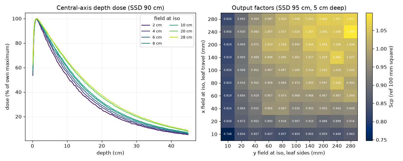
Central-axis depth doses for a sweep of square fields, and the rectangular output-factor matrix

commissioning_vsm_example.py runs a full beam-data commissioning session: a water phantom at a stated SSD, square fields, and the outputs a commissioning report carries — depth doses with dmax and PDD(10), lateral profiles in both principal directions at five depths, diagonals of the largest field, field widths and penumbrae, and a rectangular x-by-y output-factor matrix. Every error bar is the spread of independent replicates, so the nonlinear quantities carry one too. It is a jupytext percent notebook — open it as a notebook or run it as a script; the whole configuration is the parameters cell at the top.

The head is jawless with two stacked, staggered MLC layers (29 and 28 leaf pairs of 1 cm projected pitch, offset by half of it), built from published data about the Varian Halcyon and driven by an unflattened beam. Leaf ends make the inplane edge and leaf sides make the crossplane one, so a symmetric field steps in 1 cm even though each edge lands on a 0.5 cm lattice. That machine was chosen because it leaves the collimator doing everything, with no jaw to hide behind. Two results it establishes: field widths reproduce to within 0.1 mm at the isocentre with no fitted leaf-position offset, from the rounded-end tangent geometry plus a solved radiation-edge correction (the tangent ray grazes the tip, so it marks full transmission rather than the 50 % edge — worth under 0.02 mm below a 10 x 10 field and 0.84 mm at 28 x 28); and on an unflattened beam the field edge must be taken at the profile's inflection point rather than at 50 % of the axis, because the classical construction reports a 40 mm penumbra that describes the cone rather than the collimator.

The source comes one of two ways. By default it is the analytic model built in the notebook — a spectrum, a focal spot, a radial fluence, an extra-focal term and a contaminant-electron term — and needs no external data; most of that machine's geometry is unpublished, so the opening cell is an explicit inventory of what is stated, fitted, bounded or invented, and the fitted off-axis fluence table does not ship because it is derived from vendor measurements (PRIMARY_FLUENCE_FILE is the hook for one you fit against your own). Point PHASESPACE at an IAEA pair instead — or set HALCYON_VSM_PHASESPACE in the environment and run it unedited — and the whole source model arrives already sampled in the particles, leaving the notebook to supply only the collimator. That is the interesting comparison: a virtual source model fitted through some other code's simplified collimator, pushed through an explicit one. Before transporting anything that route rebuilds the model's stated spectrum and refuses the file if the records disagree by more than 50 keV in on-axis mean energy, because a phase space that contradicts its own documentation is a wasted run at best — a check that has already earned its place. No phase space ships with the repository.

Where to go next¶

Validation status — what has actually been gated, and against what.
API reference — the supported surface.